1 item has been added to your cart.

This page contains only historical information and is not about the current release of Stata. Please see our Stata 18 page for information on the current version of Stata.

Linear mixed models

Stata’s new mixed-models estimation makes it easy to specify and to fit two-way, multilevel, and hierarchical random-effects models.

To fit a model of SAT scores with fixed coefficient on x1 and random coefficient on x2 at the school level, and with random intercepts at both the school and class-within-school level, you type

 	. xtmixed sat x1 x2 || school: x2 || class: 

Estimation is either by ML or REML, and standard errors and confidence intervals (in fact, the full covariance matrix) are estimated for all variance components.

xtmixed provides four random-effects variance structures—identity, independent, exchangeable, and unstructured—and you can combine them to form even more complex block-diagonal structures.

After estimation, you can obtain best linear unbiased predictions (BLUPs) of random effects and of conditional means (fitted values).

For details, see [XT] xtmixed.

After estimation with xtmixed,

• estat recovariance reports the estimated variance–covariance matrix of the random effects for each level.
  
  
• estat group summarizes the composition of the nested groups, providing minimum, average, and maximum group size for each level in the model.
  
  predict after xtmixed can compute best linear unbiased predictions (BLUPs) for each random effect. It can also compute the linear predictor, the standard error of the linear predictor, the fitted values (linear predictor plus contributions of random effects), the residuals, and the standardized residuals.

Here are some examples from the xtmixed manual entry.

Example 1: One-level model

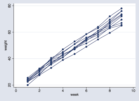
Consider a longitudinal dataset used by both Ruppert, Wand, and Carroll (2003) and Diggle et al. (2002), consisting of weight measurements of 48 pigs on nine successive weeks. Pigs are identified by variable id. Below is a plot of the growth curves for the first ten pigs.

. use http://www.statapress.com/data/r9/pig (Longitudinal analysis of pig weights) . twoway scatter weight week if id<=10, connect(L)

It seems clear that each pig experiences a linear trend in growth, and that overall weight measurements vary from pig to pig. Because we are not really interested in these particular 48 pigs per se, we instead treat them as a random sample from a larger population and model the between-pig variability as a random effect or, equivalently, as a random-intercept term at the pig level. We thus wish to fit the following model

          weight_ij = b_0 + b_1 week_ij + u_i + e_ij                 (3)

for i = 1,...,48 and j = 1,...,9. The fixed portion of the model, b_0 + b_1*week_ij, simply states that we want one overall regression line representing the population average. The random effect u_i serves to shift this regression line up or down for each pig. Since the random effects occur at the pig-level, we fit the model by typing

. xtmixed weight week || id: Performing EM optimization: Performing gradient-based optimization: Iteration 0: log restricted-likelihood = -1016.8984 Iteration 1: log restricted-likelihood = -1016.8984 Computing standard errors: Mixed-effects REML regression Number of obs = 432 Group variable: id Number of groups = 48 Obs per group: min = 9 avg = 9.0 max = 9 Wald chi2(1) = 25271.50 Log restricted-likelihood = -1016.8984 Prob > chi2 = 0.0000 ------------------------------------------------------------------------------ weight | Coef. Std. Err. z P>|z| [95% Conf. Interval] -------------+---------------------------------------------------------------- week | 6.209896 .0390633 158.97 0.000 6.133333 6.286458 _cons | 19.35561 .603139 32.09 0.000 18.17348 20.53774 ------------------------------------------------------------------------------ ------------------------------------------------------------------------------ Random-effects Parameters | Estimate Std. Err. [95% Conf. Interval] -----------------------------+------------------------------------------------ id: Identity | sd(_cons) | 3.891253 .4143198 3.158334 4.794252 -----------------------------+------------------------------------------------ sd(Residual) | 2.096356 .0757444 1.953034 2.250195 ------------------------------------------------------------------------------ LR test vs. linear regression: chibar2(01) = 473.15 Prob >= chibar2 = 0.0000 . estimates store randint

At this point, a guided tour of the model specification and output is in order:

1. By typing "weight week" we specified the response, weight, and the fixed portion of the model in the same way we would if we were using regress or any other estimation command. Our fixed effects are a coefficient on week and a constant term.
   
   
2. When we added "|| id:", we specified random effects at the level identified by group variable id, i.e., the pig-level. Since we only wanted a random intercept, that is all we had to type.
   
   
3. The output title informs us that our model was fitted using REML, the default. For ML estimates, use option mle. Since this model is a simple random-intercept model, specifying option mle would be equivalent to using xtreg, also with option mle.
   
   
4. The first estimation table is for the fixed effects. We estimate b_0 = 19.36 and b_1 = 6.21.
   
   
5. The second estimation table shows the estimated variance components. Since we only have one random effect at this level, xtmixed knew that the Identity covariance structure is the only one that makes sense. In any case, sigma_u is estimated as 3.89 with standard error 0.414.
   
   If you prefer variance estimates, e.g., sigma^2_u, to standard deviation estimates, e.g., sigma_u, specify option variance, either at estimation or upon replay.
   
   
6. The row labeled "sd(Residual)" displays the estimated standard deviation of the overall error term, i.e., sigma_epsilon = 2.10.
   
   
7. Finally, a likelihood-ratio test comparing the model to ordinary linear regression is provided and is highly significant for these data.

Example 2: One-level model

Extending (3) to also allow for a random slope on week yields the model

        weight_ij = b_0 + b_1 week_ij + u_oi + u_1i week_ij + e_ij   (4)

fitted using xtmixed

. xtmixed weight week || id: week Performing EM optimization: Performing gradient-based optimization: Iteration 0: log restricted-likelihood = -870.51473 Iteration 1: log restricted-likelihood = -870.51473 Computing standard errors: Mixed-effects REML regression Number of obs = 432 Group variable: id Number of groups = 48 Obs per group: min = 9 avg = 9.0 max = 9 Wald chi2(1) = 4592.10 Log restricted-likelihood = -870.51473 Prob > chi2 = 0.0000 ------------------------------------------------------------------------------ weight | Coef. Std. Err. z P>|z| [95% Conf. Interval] -------------+---------------------------------------------------------------- week | 6.209896 .0916386 67.77 0.000 6.030287 6.389504 _cons | 19.35561 .4021142 48.13 0.000 18.56748 20.14374 ------------------------------------------------------------------------------ ------------------------------------------------------------------------------ Random-effects Parameters | Estimate Std. Err. [95% Conf. Interval] -----------------------------+------------------------------------------------ id: Independent | sd(week) | .6135471 .0673971 .4947035 .7609409 sd(_cons) | 2.630132 .302883 2.098719 3.296105 -----------------------------+------------------------------------------------ sd(Residual) | 1.26443 .0487971 1.172317 1.363781 ------------------------------------------------------------------------------ LR test vs. linear regression: chi2(2) = 765.92 Prob > chi2 = 0.0000 Note: LR test is conservative and provided only for reference . estimates store randslope

Since we didn’t specify a covariance structure for the random effects (u_0i, u_1i), xtmixed used the default Independent structure and estimated sigma_u0 = 2.63 and sigma_u1 = 0.61. Our point estimates of the fixed effects are, for all intents and purposes, identical, but this does not hold generally. Given the 95% confidence interval for sigma_u1, it would seem that the random slope is significant, and we can use lrtest to verify this fact:

. lrtest randslope randint Likelihood-ratio test LR chibar2(01) = 292.77 (Assumption: randint nested in randslope) Prob > chibar2 = 0.0000 Note: LR tests based on REML are valid only when the fixed-effects specification is identical for both models

Example 3: Two-level model

Baltagi, Song, and Jung (2001) estimate a Cobb–Douglas production function examining the productivity of public capital in each state’s private output. Originally provided by Munnell (1990), the data were recorded over the period 1970–1986 for 48 states grouped into nine regions.

. webuse productivity (Public Capital Productivity) . describe Contains data from http://localpress.stata.com/data/r9/productivity.dta obs: 816 Public Capital Productivity vars: 11 29 Mar 2005 10:57 size: 32,640 (96.9% of memory free) (_dta has notes) ------------------------------------------------------------------------------- storage display value variable name type format label variable label ------------------------------------------------------------------------------- state byte %9.0g states 1-48 region byte %9.0g regions 1-9 year int %9.0g years 1970-1986 public float %9.0g public capital stock hwy float %9.0g log(highway component of public) water float %9.0g log(water component of public) other float %9.0g log(bldg/other component of public) private float %9.0g log(private capital stock) gsp float %9.0g log(gross state product) emp float %9.0g log(non-agriculture payrolls) unemp float %9.0g state unemployment rate ------------------------------------------------------------------------------- Sorted by:

Since the states are nested within regions, we fit a two-level mixed model with random intercepts at both the region and at the state-within-region levels.

. xtmixed gsp private emp hwy water other unemp || region: || state: Performing EM optimization: Performing gradient-based optimization: Iteration 0: log restricted-likelihood = 1404.7101 Iteration 1: log restricted-likelihood = 1404.7101 Computing standard errors: Mixed-effects REML regression Number of obs = 816 ----------------------------------------------------------- | No. of Observations per Group Group Variable | Groups Minimum Average Maximum ----------------+------------------------------------------ region | 9 51 90.7 136 state | 48 17 17.0 17 ----------------------------------------------------------- Wald chi2(6) = 18382.39 Log restricted-likelihood = 1404.7101 Prob > chi2 = 0.0000 ------------------------------------------------------------------------------ gsp | Coef. Std. Err. z P>|z| [95% Conf. Interval] -------------+---------------------------------------------------------------- private | .2660308 .0215471 12.35 0.000 .2237993 .3082624 emp | .7555059 .0264556 28.56 0.000 .7036539 .8073579 hwy | .0718857 .0233478 3.08 0.002 .0261249 .1176464 water | .0761552 .0139952 5.44 0.000 .0487251 .1035853 other | -.1005396 .0170173 -5.91 0.000 -.1338929 -.0671862 unemp | -.0058815 .0009093 -6.47 0.000 -.0076636 -.0040994 _cons | 2.126995 .1574864 13.51 0.000 1.818327 2.435663 ------------------------------------------------------------------------------ ------------------------------------------------------------------------------ Random-effects Parameters | Estimate Std. Err. [95% Conf. Interval] -----------------------------+------------------------------------------------ region: Identity | sd(_cons) | .0435471 .0186292 .0188287 .1007161 -----------------------------+------------------------------------------------ state: Identity | sd(_cons) | .0802737 .0095512 .0635762 .1013567 -----------------------------+------------------------------------------------ sd(Residual) | .0368008 .0009442 .034996 .0386987 ------------------------------------------------------------------------------ LR test vs. linear regression: chi2(2) = 1162.40 Prob > chi2 = 0.0000 Note: LR test is conservative and provided only for reference

Some items of note:

1. Our model now has two random-effects equations, separated by ||. The first is a random intercept (constant-only) at the region level, the second a random intercept at the state level. The order in which these are specified (from left to right) is significant—xtmixed assumes that state is nested within region.
   
   
2. The variance component estimates are now organized and labeled according to level. After adjusting for the nested-level error structure, we find that the highway and water components of public capital had significant positive effects upon private output, while the other public buildings component had a negative effect.

References

Baltagi, B. H., S. H. Song, and B. C. Jung. 2001.

Journal of Econometrics 101: 357–381.

Munnell, A. 1990.

Why has productivity growth declined? Productivity and public investment.

New England Economic Review. Jan. / Feb.:3–22.

Diggle, P. J., P. Heagerty, K.-Y. Liang, and S. L. Zeger. 2002.

Analysis of Longitudinal Data. 2nd edition. Oxford: Oxford University Press.

Ruppert, D., M. P. Wand, and R. J. Carroll. 2003.

Semiparametric Regression. Cambridge: Cambridge University Press.