1 item has been added to your cart.

Dynamic panel-data (DPD) analysis

Stata has a suite of commands for dynamic panel-data analysis:

• Command xtabond implements the Arellano and Bond estimator, which uses moment conditions in which lags of the dependent variable and first differences of the exogenous variables are instruments for the first-differenced equation.
• Command xtdpdsys implements the Arellano and Bover/Blundell and Bond system estimator, which uses the xtabond moment conditions and moment conditions in which lagged first differences of the dependent variable are instruments for the level equation.
• Command xtdpd, for advanced users, is a more flexible alternative that can fit models with low-order moving-average correlations in the idiosyncratic errors and predetermined variables with a more complicated structure than allowed with xtabond and xtdpdsys.
• Postestimation tools allow you to test for serial correlation in the first-differenced residuals and test the validity of the overidentifying restrictions.

Example

Building on the work of Layard and Nickell (1986), Arellano and Bond (1991) fit a dynamic model of labor demand to an unbalanced panel of firms located in the United Kingdom. First we model employment on wages, capital stock, industry output, year dummies, and a time trend, including one lag of employment and two lags of wages and capital stock. We will use the one-step Arellano–Bond estimator and request their robust VCE:

    . use http://www.stata-press.com/data/r11/abdata
    . xtabond n L(0/2).(w k) yr1980-yr1984 year, vce(robust)

Because we included one lag of n in our regression model, xtabond used lags 2 and back as instruments. Differences of the exogenous variables also serve as instruments.

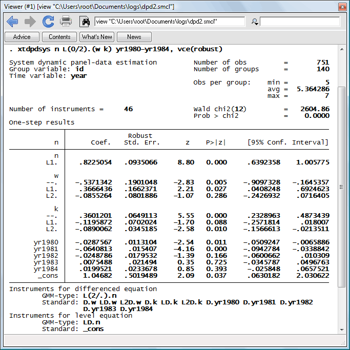
Here we refit our model, using the xtdpdsys command instead so that we can obtain the Arellano–Bover/Blundell–Bond estimates:

    . xtdpdsys n L(0/2).(w k) yr1980-yr1984 year, vce(robust)

Comparing the footers of the two commands’ output illustrates the key difference between the two estimators. xtdpdsys included the lagged differences of n as instruments in the level equation; xtabond did not.

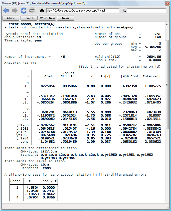
The moment conditions of these GMM estimators are valid only if there is no serial correlation in the idiosyncratic errors. Because the first difference of white noise is necessarily autocorrelated, we need only concern ourselves with second and higher autocorrelation. We can use estat abond to test for autocorrelation:

    . estat abond, artests(4)

References

Arellano, M., and S. Bond. 1991.

Some tests of specification for panel data: Monte Carlo evidence and an application to employment equations. The Review of Econometric Studies 58: 277–297.

Layard, R., and S. J. Nickell. 1986.

Unemployment in Britain. Economica 53: 5121–5169.

Back to highlights