In the spotlight: Adding your own methods to analyze power and sample size
Stata 13 added a suite of power commands to analyze power and sample size. Stata 13.1 extends that suite to ANOVA.
In some cases, you may want to compute sample size or power yourself. For example, you may need to do this by simulation, or you may want to use a method that is not available in any software package. power makes it easy for you to add your own method. All you need to do is to write a program that computes sample size, power, or effect size, and the power command will do the rest for you. It will deal with the support of multiple values in options and with automatic generation of graphs and tables of results.
Suppose you want to add the method called mymethod to the power command. Just follow these three steps:
- Create a program that computes sample size, power, or effect size and follows power’s naming convention: power_cmd_mymethod.ado.
- Store results following power’s simple naming conventions for results. For example, store the value of power in r(power), the value of sample size in r(N), and so on.
- Place your program power_cmd_mymethod.ado where Stata can find it.
To show how easy this all is, we’ll write an ado program to compute power for a one-sample z test given sample size, standardized difference, and significance level. For simplicity, we assume a two-sided test.
We will call our new method myztest.
program power_cmd_myztest, rclass
    version 13.1
                            //  parse options
    syntax , n(integer)     /// sample size
             STDDiff(real)  /// standardized diff.
             Alpha(string)  /// significance level

                            //  compute power
    tempname power
    scalar `power' = normal(`stddiff'*sqrt(`n') - ///
                     invnormal(1-`alpha'/2))

                            // return results
    return scalar power   = `power'
    return scalar N       = `n'
    return scalar alpha   = `alpha'
    return scalar stddiff = `stddiff'
end
The computation in this program takes only one line, but it could be as complicated as we like. It could even involve simulation to compute the power.
With our program in hand, we can type
. power myztest, n(20) stddiff(1) alpha(.05)
power will find our ado program, supply it with the options n(20), stddiff(1), and alpha(.05), and use its returned results to produce
. power myztest, n(20) stddiff(1) alpha(.05)

Estimated power
Two-sided test
| alpha power N | |||
| .05 .994 20 | |||
That wasn’t too impressive. Our program did all the work.
But what if we supplied power with a list of sample sizes?
. power myztest, n(10 15 20 25) stddiff(1)

Estimated power
Two-sided test
| alpha power N | |||
| .05 .8854 10 | |||
| .05 .9721 15 | |||
| .05 .994 20 | |||
| .05 .9988 25 | |||
power has taken our list of sample sizes and computed powers for all of them—even though our program could only compute a single power!
Moreover, we can use power’s standard table() option to control exactly how that table looks. power also has hooks that let our program determine how the columns are labeled and how the table appears.
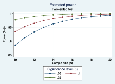
We can supply both sample sizes and significance levels and request a graph instead of a table:
. power myztest, n(10(1)20) alpha(.05 .10 .25) stddiff(1) graph

We can even request that the graph show α on the x axis with separate plots for each sample size.
. power myztest, n(10(2)20) alpha(.05 .10 .25) stddiff(1) graph(xdim(alpha))

Now all this may just make it worth writing more complicated programs to compute power for more complicated tests and comparisons.
We had room here to do just a simple example. More details and extensions of this example are covered in my presentation, Power of the power command, at the 2013 UK Stata Users Group meeting. Complete documentation for user-programed power and sample size can be found in Stata 13.1 by typing help power userwritten.
— Yulia Marchenko
Director of Biostatistics


