1 item has been added to your cart.

Generalized method of moments (GMM)

Stata’s new gmm command makes generalized method of moments estimation as simple as nonlinear least-squares estimation and nonlinear seemingly unrelated regression. Just specify your residual equations by using substitutable expressions, list your instruments, select a weight matrix, and obtain your results.

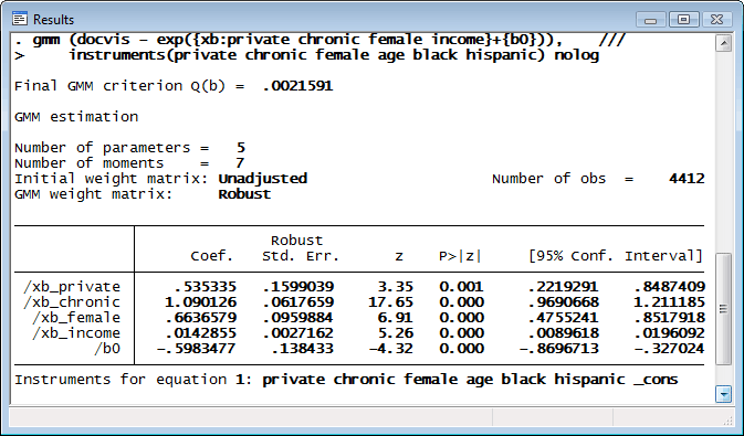
Here we fit a Poisson model of the number of doctor visits as a function of gender, income, and whether a person has a chronic disease or private health insurance. We have reason to believe that income is endogenous, so we use age and race as instruments.

By default, gmm uses the two-step estimator and a weight matrix that assumes the errors are independent but not identically distributed. By using the wmatrix() and vce() options, you can request weight and variance–covariance matrices appropriate for errors that are independent and identically distributed, are independent but not identically distributed, exhibit group-level clustering, or that exhibit heteroskedasticity and autocorrelation. In addition, you can obtain standard errors via the bootstrap or the jackknife.

When fitting a model by GMM, you should check to see whether the instruments you use really satisfy the orthogonality condition—i.e., whether they are uncorrelated with the errors. In GMM estimation, Hansen’s J statistic is the most common test statistic. In our example, whether our instruments are valid is certainly open for debate—age likely influences the number of doctor visits—and we can test their validity by using estat overid to obtain Hansen’s J statistic:

The test statistic has a χ² distribution under the null hypothesis that the instruments are valid. The significant statistic indicates that one or more of our instruments are not valid (assuming that the model is otherwise correctly specified).

gmm’s numerical derivative routines are very accurate, so most of the time you do not need to spend time taking analytic derivatives. However, if speed is of the essence or if you plan to fit the same model repeatedly, analytic derivatives can be a boon. gmm provides a simple way to specify derivatives. We could fit our previous model with analytic derivatives by specifying

The notation {xb:private chronic female income} is a shorthand to create a linear combination of variables; we could have specified {xb_private}*private + {xb_chronic}*chronic + {xb_female}*female + {xb_income}*income and declared each parameter explicitly. By using the shorter notation, we need only specify the derivative with respect to the entire linear combination instead of each parameter individually. Moreover, once we declare our linear combination, we can subsequently refer to it as xb: without having to specify the variables associated with it.

In addition to standard instruments, gmm allows you to create panel-style instruments used in dynamic and other panel models with endogenous regressors. In these models, you typically use lagged values of regressors as instruments; the number of lagged values available increases as the time dimension increases. gmm’s xtinstruments() option makes creating these instruments a snap.

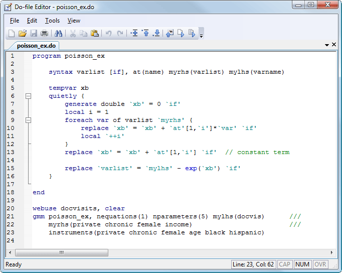
For more complicated analyses, gmm allows you to write a program to evaluate your residual equations instead of using substitutable expressions. These programs are structured like those that ml, nl, and nlsur use. Here is our Poisson model fit using the moment-evaluator program version of gmm:

The programmable version of gmm is eminently flexible. You just need to tell it how many moment equations you have and the number of parameters in your model. You can optionally specify instruments and select the type of weight matrix to use and standard errors to report.

Explore more about gmm in Stata.

Back to highlights