1 item has been added to your cart.

New univariate time-series features added in 13.1

Stata 13.1 introduces four new features for univariate time series:

1. IRFs (impulse–response functions) for ARIMA and ARFIMA models
2. Parametric autocorrelation estimates from ARIMA and ARFIMA models
3. A check of stability conditions for ARIMA models
4. Spectral density estimation from seasonal ARIMA models

Individually, none of these features are earth shattering. However, the first three are some of my go-to concepts when teaching time-series analysis. Let’s use an example to see why.

Here is a graph of changes in monthly U.S. civilian unemployment rates for the period 1948–2011.

We fit an ARIMA model with two autoregressive (AR) terms, first-differencing, and no moving-average terms.

. arima unrate, arima(2,1,0)

ARIMA regression

Sample:  1948m2 - 2011m1                        Number of obs      =       756
                                                Wald chi2(2)       =    101.75
Log likelihood =  124.1939                      Prob > chi2        =    0.0000



             
 
                 OPG

    D.unrate 
 
      Coef.   Std. Err.      z    P>|z|     [95% Conf. Interval]

 
 
 

unrate       
 
 

       _cons 
 
   .0072595   .0127559     0.57   0.569    -.0177417    .0322606

 
 
 

ARMA         
 
 

          ar 
 
 

         L1. 
 
   .0887064   .0224304     3.95   0.000     .0447437    .1326691

         L2. 
 
   .2897793   .0330048     8.78   0.000     .2250911    .3544675

 
 
 

      /sigma 
 
   .2052886   .0032441    63.28   0.000     .1989304    .2116469


Note: The test of the variance against zero is one sided, and the two-sided
    confidence interval is truncated at zero.

The AR parameters are statistically significant, and they indicate a moderate degree of temporal dependence.

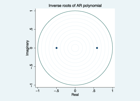
Inference after ARIMA requires that the ARMA (autoregressive moving-average) process be covariance stationary. The stationarity of an ARMA process depends on the AR parameters. The inverse roots of the AR polynomial must all lie inside the unit circle for the process to be stationary. We use the new estat aroots command to examine this requirement:

. estat aroots

   Eigenvalue stability condition


  
        Eigenvalue        
 
   Modulus   


   
 
 
 


  
   .5844888               
 
   .584489   


  
  -.4957824               
 
   .495782   



   All the eigenvalues lie inside the unit circle.
   AR parameters satisfy stability condition.

The ARMA process appears to be stationary because both inverse AR roots lie well inside the unit circle.

A crucial aspect of time-series processes are their autocorrelations. The autocorrelations provide a scale-free measure of the dependence structure of the process. We can obtain a graph of this structure using the new estat acplot command after estimating our ARIMA model:

. estat acplot, lags(10)

The graph shows that the autocorrelations decay exponentially toward 0, which is typical of a stationary AR process with positive coefficients.

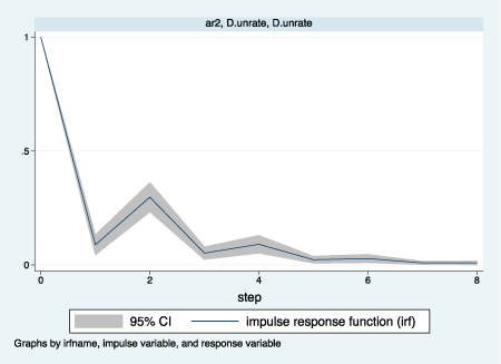
We often want to know how an exogenous shock feeds through our model and affects the series. This response, measured over time, is called the impulse–response function (IRF).

We create an IRF for our ARIMA model by typing

. irf create ar2, set(myirf)

and then graph that IRF by typing

. irf graph irf

The trajectory of the IRF shows that a positive shock initially causes an increase in unemployment but that the increase nears 0 by 5 months and completely dies out after 7 or 8 months.

You can see more examples of these new facilities in the manuals. See arima postestimation and arfima postestimation.

—Rafal Raciborski
Senior Statistical Developer